Hypothesis testing 3

Recall, from Hypothesis testing 2, the problem

The fuel efficiency, in miles per gallon, of the Vauxwagen Etcetera is \mu _{0}=38.5 with a known standard deviation of \sigma _{0}=3.2. The company claims that it has improved the fuel efficiency of its latest model, and in support of that claim cites evidence from the testing of ten new cars under normal conditions; the new cars had an average fuel efficiency of m=40.3 miles per gallon.

How good is the evidence for the company's claim?

We originally solved this problem by noting that the test statistic

is distributed N(0,1). Its value is 1.778, and

meaning that if the null hypothesis were true, it is unlikely that the difference would be ths extreme (or more) through pure random variation.

In fact, that's not usually how we do things. Instead, we decide in advance what the cutoff point for unlikely ought to be (0.05 is pretty common, but not universal), and then find the value of the test statistic associated with that probability (which we call the critical value).

If the actual value is more extreme (that is, further from zero) than this critical value, then we regard the effect as significant and reject the null hypothesis.

Let's make 0.05 our cutoff point for this problem (this is called testing at the 5% level). We're then after the value z such that

or (equivalently)

This turns out to be 1.645. Since the actual value is more extreme than this, we reject the null hypothesis: the fuel efficiency really does seem to have improved.

Note, though, that testing at the 5% level is pretty arbitrary. If we need stronger evidence, we could (for example) test at the 2% level. In this case, the critical value is the value of z such that

which is 2.054. The actual value of our test statistic is less extreme than this, meaning that we would accept the null hypothesis at the 2% level.

In general, the smaller the level, the sterner the test of the alternative hypothesis: that is, the stronger the evidence we require before rejecting the null hypothesis.

Two-tailed tests

Consider the following problem

A study is carried out into the effects of music on concentration. Twenty volunteers were sorted, as homogenously as possible, into two groups, and made to perform a corpus of 40 mental tasks. The first group worked with loud hip-hop in the background, whereas the second worked to equally loud metal.  The scores out of 40 in the first group were 21, 19, 25, 23, 29, 22, 22, 24, 23 and 22. Those in the second group were 23, 20, 16, 21, 18, 21, 29, 20, 25 and 19. Test at the 5% level whether there is any significant difference. You may assume a common standard deviation.

Here, we're testing the difference between two means, with standard deviations estimated from the samples. The means are m_{1}=23.0 and m_{2}=21.2 respectively, and the sample standard deviations are 2.67 and 3.71 respectively. The common standard deviation is

and the test statistic is

which is distributed

The value of the test statistic is 1.247.

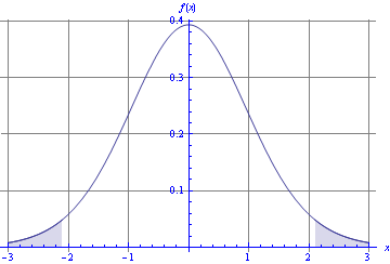
Now, here's the difference between this situation and the previous one. Before, we were interested in testing whether there had been an improvement: that is, a directional change. Here, we want to test whether there has been a change of any kind: that is, a change in either direction. This is called a two-tailed test.

To carry out a two-tailed test at the 5% level, we need to find the values of x such that, for a random variable T\sim t(18),

Figure 1 illustrates the region concerned (known as the critical region).

Figure 1: Critical region for a two-tailed t-test at the 5% level

This is clearly the same as finding that value of x for which

or indeed

This critical value turns out to be 2.101, and our actual value is less extreme; there is no good evidence for a difference.

Tabulations

To carry out one-tailed tests at the 5% level, we need the 95th percentage point of all the t-distributions up to t(30), plus that of N(0,1).

To carry out two-tailed tests at the 5% level, we need the 97.5th percentage point of all the t-distributions up to t(30), plus that of N(0,1).

To carry out one-tailed tests at the 2% level, we need the 98th percentage point of all the t-distributions up to t(30), plus that of N(0,1).

To carry out two-tailed tests at the 2% level, or one-tailed tests at the 1% level, we need the 99th percentage point of all the t-distributions up to t(30), plus that of N(0,1).

To carry out two-tailed tests at the 1% level, we need the 99.5th percentage point of all the t-distributions up to t(30), plus that of N(0,1).