Motion under uniform acceleration

Consider a particle moving with a constant acceleration, a\,\text{m}\,\text{s}^{-2}. If its initial speed is u\,\text{m}\,\text{s}^{-1}, then after t seconds its speed v is given by

v=u+a\,t.

Simple integration tells us that the distance it travels in this time, s\,\text{m}, is given by

s=u\,t+\frac{1}{2}a\,t^{2}.

Squaring both sides of the first equation gives

v^{2}=u^{2}+2a\,u\,t+a^{2}t^{2}

that is,

v^{2}=u^{2}+2a(u\,t+\frac{1}{2}a\,t^{2})

or simply

v^{2}=u^{2}+2\,a\,s.

These three kinematics equations can be used to study motion under uniform acceleration. However, it's often easier instead to work graphically, noting that:

acceleration is the gradient of the velocity-time graph;

distance travelled is the area under the velocity-time graph.

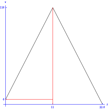
For example, consider the following problem. A vehicle accelerates uniformly from 6 metres per second at time t = 0 to 116 metres per second, taking 11 seconds to do so. Given that it then decelerates uniformly to rest, taking 11.6 seconds to do so, calculate the total distance travelled, in metres, between time t = 0 and coming to rest.

This motion is illustrated in Figure 1.

Figure 1: velocity-time sketch for the motion above

The distance we require is the area of a rectangle plus that of two triangles; it's simply

s=11\times 6+\frac{1}{2}\times 11\times 110+\frac{1}{2}\times 11.6\times 116=1343.8\,\text{metres}.