The complex number z=x+i\,y can be represented in the Argand diagram by the vector $$\left[ \begin{array}{c}x\\y \end{array}\right],$$ and the argument of z, written \arg z, is simply the direction of this vector. This direction is expressed as the angle from the horizontal axis to the vector representing z, with anticlockwise being the positive direction.
In order to ensure that every complex number has a unique argument, the argument of a complex number always lies within a certain interval of length 2\pi. Two conventions exist: some mathematicians insist that $$0\le\arg z<2\pi,$$ and others that $$-\pi<\arg z\le \pi.$$ Note that $$\tan \,(\arg z)=\frac{y}{x},$$ but that it is not always the case that $$\arg z = \tan^{-1} \frac{y}{x}.$$ In the figure, for example, which shows the complex number $$z=-1+\sqrt{3}\,i,$$ the argument is 2\pi/3 radians, whose tangent is -\sqrt{3}; however, $$\tan^{-1}(-\sqrt{3})=-\pi/3\ne2\pi/3.$$
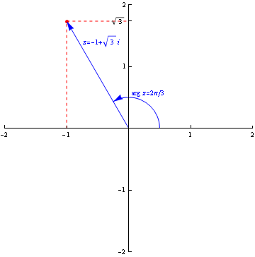
Figure 1: The argument of a complex number: \arg(-1+\sqrt{3}\,i)=2\pi/3
An arithmetic sequence (or series) is a sequence (or series) in which each term is obtained from the last by addition of a constant quantity (known as the common difference). For example, $$1,3,5,7,9,\dots$$ is an arithmetic sequence and $$1+3+5+7+9+\dots$$ is the corresponding series: the common difference is 2.
Consider a data set consisting of coordinate pairs, and suppose that it's known, or at least conjectured, that this data reflects a certain kind of relationship between the variables: a linear one, perhaps, or a quadratic one (this "relationship type'' is called the model).
Suppose we wish to find the relationship between the variables, as best we can. However, suppose that measurement error, or some other source of "noise", makes each data point's location slightly imprecise. Then there may be no curve conforming to the model that exactly fits the data, in which case what we want is a curve that accords with our model and that (in some sense) fits the data "best''.
What we usually mean by "best'' is the least squares best fit curve, in which the curve is chosen, from among all those allowed by our model, to minimise the sum of the squares of the vertical distances between the data and the curve. The figure shows some data together with its least squares best fit quadratic; the vertical distances (which are known as residuals) are also shown.
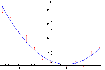
Figure 1: A data set (red) together with a least squares best fit quadratic curve (blue),
showing vertical distances or residuals (pink)
A bounded region in a space is one all of whose points lie within a set finite distance from some point of the space. In two dimensions, this means we can draw a circle round it (in three dimensions, a sphere, and so on).
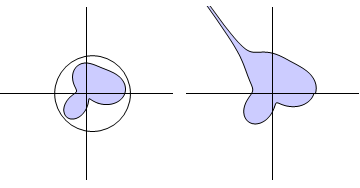
Figure 1: Bounded and unbounded sets in two dimensions
A function is bounded on its domain if all its values lie within a set finite distance of some particular value. In graphical terms, this means we can enclose the function's graph within parallel "tramlines''.
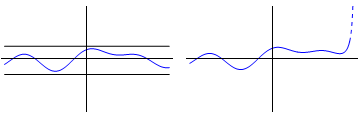
Figure 1: Bounded and unbounded functions on a finite domain
When two flat surfaces are in contact, the force between them consists of a normal reaction, N, at right angles to the surfaces, and a frictional reaction, F, parallel to them (see Figure 1). The frictional reaction exactly balances any force that is applied parallel to the surfaces; or rather, this happens up to a certain maximum value of the applied force, above which the surfaces slip. This maximum value is proportional to N, and also depends on how rough the surfaces are: the rougher the surfaces, the stronger the force that can be applied without them slipping.
We can say that F\le \mu N, where \mu, which is a measure of how rough the surfaces are, is called the coefficient of friction between them.
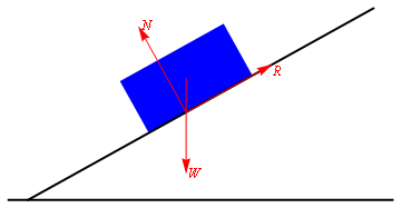
Figure 1: Two surfaces in frictional contact
The complex conjugate of the complex number $$z=x+i\,y$$ is defined to be $$\bar{z} = x-i\,y.$$ Note that z\,\bar{z} = x^2+y^2 is real, and equal to the square of z's modulus.
The non-real roots of real polynomials always occur as pairs of conjugate complex numbers.
Given a function f(x), its derivative, f'(x), is, in terms of x the gradient at the point (x, f(x)): the derivative is the "gradient function'', you might say.
For any small value of h, it is approximately given by $$\frac{f(x+h)-f(x)}{h},$$ with exact equality in the limit as h tends to zero. This is illustrated in Figure 1.
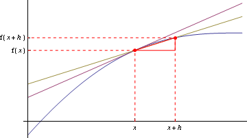
Figure 1: The idea of a derivative
An even function is a function f such that $$f(x) = f(-x)$$ for all x for which f is defined. Even functions have graphs with reflection symmetry about the y-axis: see Figure 1 below.
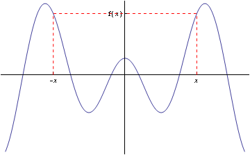
Figure 1: Graph of an even function
The differential equation $$(x^2+2\,x\,y)\,\frac{dy}{dx}+2\,x\,y+y^2=0$$ looks hard to solve, but can be written as $$\frac{d}{dx}\,(x^2\,y+x\,y^2)=0,$$ meaning that its solution is simply $$x^2\,y+x\,y^2=k,\quad\mbox{constant}.$$ Whenever a differential equation can be written in this way, in the form $$\frac{d}{dx}(\mbox{expression}) = 0,$$ we say it is exact, and the left-hand-side is called an exact derivatives.
Exact differential equations are often written in terms of differentials instead of derivatives, as in $$(2\,x\,y+y^2)\,dx+(x^2+2\,x\,y)\,dy=0.$$
A geometric sequence (or series) is a sequence (or series) in which each term is obtained from the last by multiplication by a constant quantity (known as the common ratio). For example, $$1,-2,4,-8,16,\dots$$ is an arithmetic sequence and $$1-2+4-8+16+\dots$$ is the corresponding series: the common ratio is -2.
The gradient of a straight line is how far it rises for every 1 unit travelled horizontally: the gradient of the straight line through the point (x_1, y_1) and (x_2, y_2) is $$\frac{y_2-y_1}{x_2-x_1}.$$ This is shown in Figure 1.
The gradient of a curved line changes as you go along it. At any given point, it is equal to the gradient of the straight line that just touches the curve at that point, which is know as the tangent. This is shown in Figure 2.
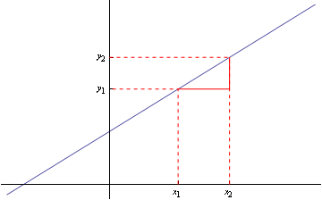
Figure 1: Gradient of a straight line
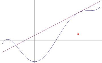
Figure 2: Gradient of a curve at a point
The Heaviside step function, H(x), is given by $$H(x)= \left\{ \begin{array}{cc} 0,&x<0,\\ 1,&x\ge 0. \end{array} \right. $$
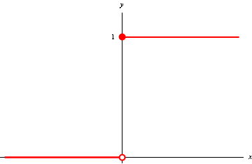
Figure 1: The Heaviside step function
The hyperbolic cosine, \cosh x, is defined as follows: $$\cosh x = \frac{e^x+e^{-x}}{2}.$$ The hyperbolic sine, \sinh x, is defined as follows: $$\sinh x = \frac{e^x-e^{-x}}{2}.$$ The hyperbolic tangent, \tanh x, is defined as follows: $$\tanh x = \frac{\sinh x}{\cosh x} =\frac{e^x-e^{-x}}{e^x+e^{-x}} .$$
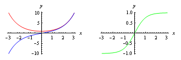
Figure 1: The hyperbolic cosine (red), sine (blue) and tangent (green)
An integral is improper if, for some reason, the region in the plane that it corresponds to is unbounded. This can happen in two ways: either the range of integration may be infinite, as in $$\int_1^{\infty}\frac{1}{x^2}\,dx,$$ or the function may have a singularity within or on the edge of the range of integration, as in $$\int_1^5\frac{1}{\sqrt{x-1}}\,dx.$$ Note that an unbounded region need not necessarily have infinite area, and if not, the integral will have a finite value (as both of these do).
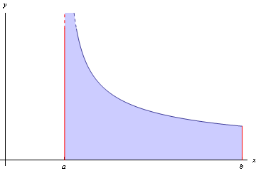
Figure 1: Improper integral: unbounded function integrated over a finite domain
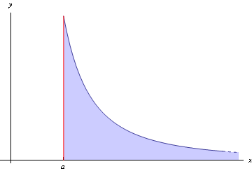
Figure 2: Improper integral: bounded function integrated over an infinite domain
The intercept of a straight line is the point where its graph crosses the y-axis. This is shown in Figure 1.
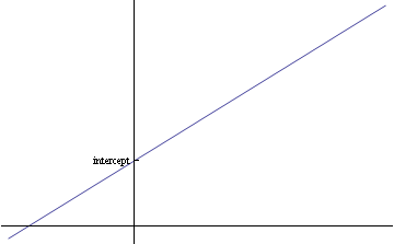
Figue 1: Intercept of a straight line
Any function f that is one-to-one (that is, for which no two inputs give the same output) has an inverse f^{-1}, which represents f ``in reverse''. That is, if $$y=f(x),$$ then $$x=f^{-1}(y),$$ for all x on which f is defined. Functions that aren't one-to-one, such as sine or cosine, can sometimes be given an inverse by considering the function only over a restricted domain.
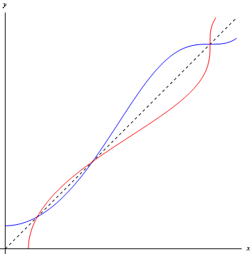
Figure 1: A function (blue) and its inverse (red)
For any collection of n+1 data points $$(x_0,y_0),\,(x_1,y_1),\,(x_2,y_2),\dots,\,(x_n,y_n)$$ (as long as none share the same x-value) there is exactly one polynomial of degree n whose graph passes through all the points. This is given by the formula $$f(x) = \sum_{i=0}^n\,y_i\,\frac{(x-x_0)\dots(x-x_{i-1})(x-x_{i+1})\dots(x-x_n)}{(x_i-x_0)\dots(x_i-x_{i-1})(x_i-x_{i+1})\dots(x_i-x_n)}.$$ Finding this polynomial is called Lagrangian interpolation.
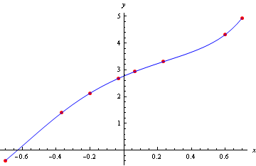
Figure 1: Lagrangian interpolation of a set of 8 data points by a polynomial
of degree 7
Consider a sequence $$a_1,\,a_2,\,a_3,\,\dots$$ Suppose that there's some number l that this sequence approaches as we take successive terms. (By this we mean something very precise, namely that we can specify a pair of values as close as we like to l, and be sure that eventually, all the terms of the sequence will lie between these values.)
We say that l is the limit of the sequence (a_n) as n tends to infinity.
We can use the same idea for functions of x: the limit of f(x) as x tends to infinity is l provided we can specify a pair of values as close as we like to l, and be sure that eventually, for large enough x, all values of f(x) lie within these values.
The same idea works for x tending to negative infinity, and we can also extend it to finite values of x. If we can specify a pair of values as close as we like to l, and be sure that as long as x lies close enough to a then f(x) lies between these values, then f(x) tends to the limit l and x tends to a.
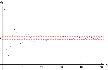
Figure 1: A sequence apparently tending to a limit l
When two flat surfaces are in contact, the force between them consists of a normal reaction, N, at right angles to the surfaces, and a frictional reaction, F, parallel to them (see Figure 1).
If the coefficient of friction between the surfaces is \mu, then F\le \mu N. If the surfaces are slipping against each other, F is always equal to \mu N.
If the surfaces are static with respect to each other, but F = \mu N, then the surfaces are on the point of slipping. This set of circumstances is called limiting friction.
Figure 1: Two surfaces in frictional contact
The inverse of an exponential function: the statement $$y = \log_a x$$ means exactly the same thing as $$x = a^y.$$ The inverse of the exponential function, e^x, is known as the natural logarithm, written \ln x (or sometimes just \log x). Its graph is shown in Figure 1.
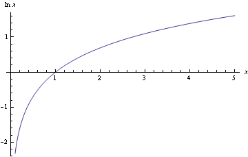
Figure 1: Graph of the natural logarithm
A maximum of a function of two variables corresponds, in a surface plot of f, to the top of a hill.
A minimum of a function f is a point that is the lowest in its immediate neighbourhood. If f is a function of one variable, then df/dx is zero at a minimum; if f is a function of more than one variable, then all its partial derivatives are zero at a minimum.
A minimum of a function of two variables corresponds, in a surface plot of f, to the bottom of a depression.
The modulus of a real number x, also called its absolute value, is written |x| and defined by $$|x| = \left\{ \begin{array}{cc} x,&x\ge 0,\\ -x,&x<0. \end{array}\right.$$
The graph of |x| is shown in Figure 1.
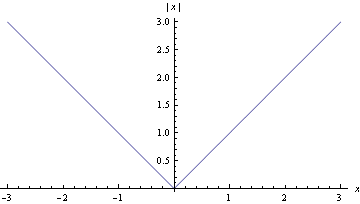
Figure 1: Graph of the modulus function
A monkey saddle is an example of a stationary point of a function of two variables that doesn't fall into any of the usual categories, being neither a maximum, nor a minimum, nor an ordinary (simple) saddle point. Such stationary points are rare, and correspond to a value of exactly zero for the test function $$z_{xx}\,z_{yy}-{z_{xy}}^2.$$ An example is the point at the origin in the surface plot of $$z=x^3-3\,x\,y^2,$$ shown in the figure.
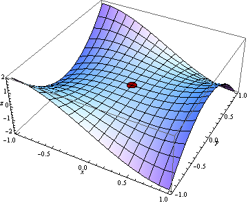
Figure 1: A monkey saddle: the point (0,0,0) on the surface plot z=x^3-3\,x\,y^2
The inverse of the exponential function, e^x; the natural logarithm is written \ln x and is defined by stating that $$y=\ln x$$ if and only if $$x=e^y.$$
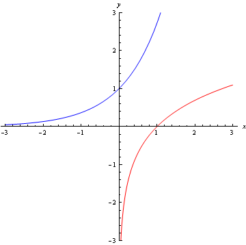
Figure 1: Plot of the exponential function y=e^x (blue) and its inverse,
the natural logarithm y=\ln x
An odd function is a function f such that $$f(x) = -f(-x)$$ for all x for which f is defined. Odd functions have graphs with rotation symmetry about the origin: see Figure 1.
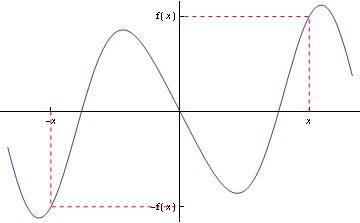
Figure 1: Graph of an odd function
A method for converting trigonometrical identities to hyperbolic identities:
- Convert every trigonometrical function to the corresponding hyperbolic function.
- Change the sign of each term containing the product of two (hyperbolic) sines.
Thus for example $$\cos2\theta=\cos^2\theta-\sin^2\theta$$ becomes $$\cosh2x=\cosh^2x+\sinh^2x.$$
The general solution of a linear differential equation $$a_0(x)+a_1(x)\,\frac{dy}{dx}+\dots+a_n\,\frac{d^ny}{dx^n}=g(x)$$ consists, in general, of two components: one that just reflects the intrinsic properties of the system and one that also reflects the way the system is driven. The latter is known as the particular integral. {\em Any} solution of the differential equation can serve as a particular integral, but the simplest is usually chosen.
If the coefficients a_0, a_1 etc are constants rather than functions of x, then the particular integral is often closely related to the driving function g(x).
Pascal's triangle is a quick way of working out the coefficients in the binomial expansion of (a+b) for smallest positive integer n. The first line of the triangle is $$1\quad\quad1$$ and each subsequent line is generated by calculating the sums of neighbouring elements of the line above (and then putting a 1 on each end). The first seven lines of Pascal's triangle are
$$\begin{array}{ccccccccccccccc} &&&&&&1&&1&&&&&&\\ &&&&&1&&2&&1&&&&&\\ &&&&1&&3&&3&&1&&&&\\ &&&1&&4&&6&&4&&1&&&\\ &&1&&5&&10&&10&&5&&1&&\\ &1&&6&&15&&20&&15&&6&&1&\\ 1&&7&&21&&35&&35&&21&&7&&1 \end{array}$$
and thus, for example, $$(1+x)^5 = 1+5x+10x^2+10x^3+5x^4+x^5.$$
A point of inflexion of a function f(x) is a point at which its gradient stops falling and starts rising, or vice versa. At any point of inflexion, f''(x) = 0 (but be careful: this can also occur at maxima or minima). The idea is illustrated in Figure 1. Note that the rightmost point of inflexion is also a stationary point, because the gradient there happens to be zero.Note, though, that neither of the other two points of inflexion are stationary points.
Note: one way to think about points of inflexion is to imagine driving a car along a road shaped like the curve. Some of the time, you're steering left, and some of the time right. Points of inflexion correspond to your steering wheel being, for that instant, exactly centred, as you cross from right steer to left steer or vice versa.
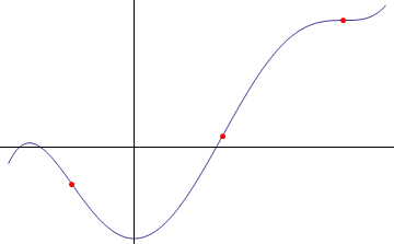
Figure 1: Points of inflexion
The position vector of a point A is the vector OA, where O is the origin: see Figure 1
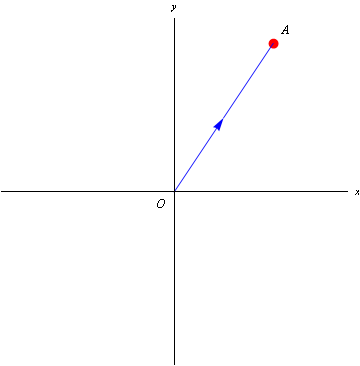
Figure 1: OA, the position vector of the point A
A simple trigonometrical equation such as $$\sin x = 0.65$$ has infinitely many solutions, because the graph of y = \sin x is periodic. One of these solutions is treated as the principal one, namely the one that happens to lie between -\pi/2 and \pi/2. This is shown in Figure 1. It is this principal value that we use when calculating \sin^{-1} 0.65.
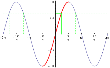
Figure 1: Principal solutions of sine equations
When the equation involves a cosine instead of a sine, the principal value lies between 0 and \pi; when a tangent, -\pi/2 and \pi/2 again. These are shown in Figures 2 and 3 respectively.
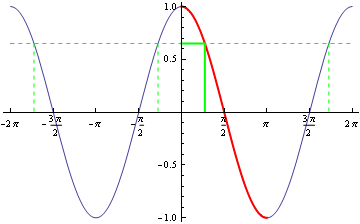
Figure 2: Principal solutions of cosine equations
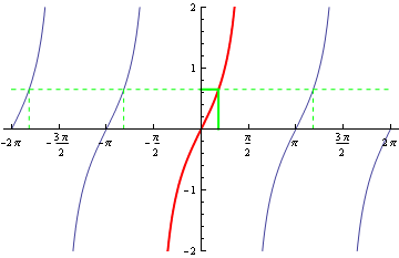
Figure 3: Principal solutions of tangent equations
The "natural'' measure of angle, used because it makes calculus with trigonometrical functions much more straightforward; for example, if x is measured in radians then $$\frac{d}{dx} (\sin x) = \cos x.$$ The angle in radians is equal to "arc length over radius''. There are 2\pi radians in a full circle.
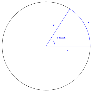
Figure 1: One radian
Maclaurin series generally converge either for all x or for -r< x< r, for some r. In the latter case, we say the radius of convergence is r; in the former, we say it is infinite. (Taylor expansions about x=a work in a similar way; either they converge for all x or they converge for a-r< x< a+r.)
The radius of convergence can be calculated by applying the ratio test: it is given by the range of x-values for which the ratio of successive terms is numerically less than 1.
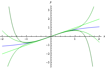
Figure 1: Plot of \arctan x (blue) together with successive Maclaurin approxomations
(darkening shades of green), showing convergence only within -1<x<1
Strictly, when defining a function, we must specify a set to which its values all belong: a set of possible "outputs''. This set is called the function's range.
Note:the terminology can get ambiguous here. Some people say that
a function's range must be precisely all its possible values, whereas
others call this set the "image'', and allow the range to be any set within
which the image is contained.
In the case of the series $$\sum_{r=1}^{\infty} \,a_r,$$ if the limit $$\lim_{r\to\infty}\,\left|\frac{a_{r+1}}{a_r}\right|$$ exists and is less than 1, then the series converges; if it exists and is greater than 1, then the series diverges; if the fraction $$\left|\frac{a_{r+1}}{a_r}\right|$$ tends to infinity, then the series diverges.
Note that if this fraction either (i) fails to converge while not tending to infinity, or (ii) converges to 1 exactly, then the ratio test tells us nothing about whether or not the series converges.
In general, a way of using two estimates for a quantity, calculated using different step sizes, to obtain a third estimate that we can expect to be better than either, using what we know about the estimates' order of convergence (see order (2)).
In the case of the trapezium rule, given two estimates T_m and T_n, calculated using m intervals and n intervals respectively, the Richardson extrapolation is $$\frac{n^2\,T_n-m^2\,T_m}{n^2-m^2}.$$ In the case of Simpson's rule, if the two estimates are S_m and S_n, then the Richardson extrapolation is $$\frac{n^4\,S_n-m^4\,S_m}{n^4-m^4}.$$
A (simple) saddle point is a stationary point of a function of two variables that is a minimum along some paths and a maximum along others. On a surface plot, it corresponds to a pass between two hills, or to a the shape of a horse-riding saddle, or to a Pringle crisp.
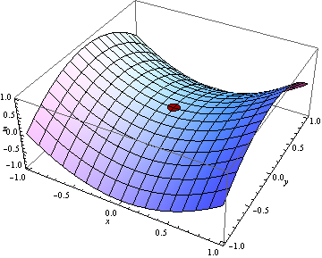
Figure 1: A simple saddle: the point (0,0,0) on the surface plot z=x^2-y^2
A numerical method for calculating the approximate value of an integral, by approximating the integrand by a sequence of quadratic polynomials. We sample the integrand at n+1 points, $$y_0,\,y_1,\,\dots,y_n,$$ where n is even; these correspond to x-values evenly spaced a distance h apart. Then the integral is given approximately by $$\frac{h}{3}\,(y_0+4\,y_1+2\,y_2+4\,y_3+2\,y_4+\dots+2\,y_{n-2}+4\,y_{n-1}+y_n).$$
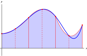
Figure 1: Simpsons's rule: numerical integration by approximating an integrand
(blue curve) with a sequence of quadratic functions (three red curves)
Two lines in three dimensions are skew if they are neither parallel nor intersecting: that is, if they "miss'' one another.
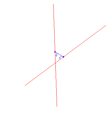
Fgiure 1: Two skew lines and the line joining their points of closest approach
A stationary point of a function f(x) is a point at which its graph is locally horizontal: that is, a point at which f'(x) = 0. The idea is illustrated in Figure 1, which shows the three types that exist: from left to right, a maximum, and minimum and a stationary point of inflexion.
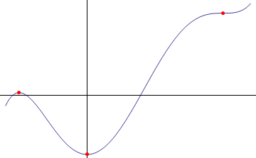
Figure 1: Stationary points: maximum, minimum and stationary point of inflexion
A function z=f(x,y) visualised as a surface in three dimensions: the coordinates x and y are treated like map references, and z then specifies a height. Mathematical surfaces resemble physical landscapes, with features like hills, depressions and mountain passes.
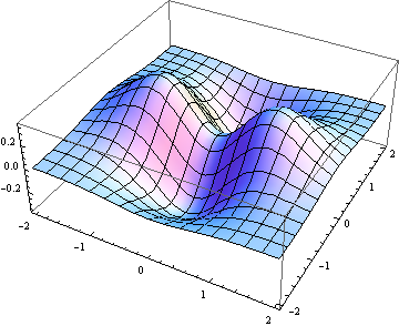
Figure 1: Surface plot of the function z=(x^2-y^2)\,e^{-x^2-y^2}
A numerical method for calculating the approximate value of an integral, by approximating the integrand by a sequence of linear functions. We sample the integrand at n+1 points, $$y_0,\,y_1,\,\dots,y_n;$$ these correspond to x-values evenly spaced a distance h apart. Then the integral is given approximately by $$\frac{h}{2}\,(y_0+2\,y_1+2\,y_2+\dots+2\,y_{n-2}+2\,y_{n-1}+y_n).$$
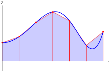
Figure 1: Trapezium rule: numerical integration by approximating an integrand
(blue curve) with a sequence of linear functions (six red line segments)
Certain structures in n-dimensional space (lines and planes, for example) can be specified by means of an equation involving the position vector of points that they contain.
The vector equation of a line is parametric, and is of the form $${\bf r} = {\bf a} + t {\bf d}.$$ In three dimensions, the vector equation of a plane is of the form $${\bf r}\cdot{\bf n}=h.$$