Our brains experience sound as rich and complex, and made up of many elements that are present at the same time; yet sound is simply a variation of pressure with time, and as such, any sound can be represented as a simple two-dimensional graph. How can both these things be true: how can a sound consist of many elements, yet be one graph?
Part of the answer is that any sound wave, or any periodic wave-like signal, can be broken down into a sum of simple sines and cosines (plus possibly a constant). This sum, which is in general infinite, is called the signal's Fourier series.
To be more precise, if f is periodic with period 2L, then we can always write
\begin{eqnarray}f(x) &=& \frac{a_0}{2} + \left\{a_1 \cos \frac{\pi x}{L} + a_2 \cos \frac{2\pi x}{L} + a_3 \cos \frac{3\pi x}{L} + \dots\right\}\\&& +\left\{b_1 \sin \frac{\pi x}{L} + b_2 \sin \frac{2\pi x}{L} + b_3 \sin \frac{3\pi x}{L} + \dots\right\} \end{eqnarray}
This series might not hold at all points, but will (in a certain sense that we can make more precise) hold at all except a small and scattered minority of such points).
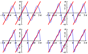
The figure shows an example. The signal, shown by the thick red line, is a sawtooth signal: f(x) is equal to x for -\pi\le <\pi, and is periodic with period 2\pi. The blue curves represent the successive approximations
\begin{eqnarray} f_1(x)&=&2\,\sin(x),\\ f_2(x)&=&2\,\left(\sin(x)-\frac{1}{2}\,\sin\,2x\right),\\ f_3(x)&=&2\,\left(\sin(x)-\frac{1}{2}\,\sin\,2x+\frac{1}{3}\,\sin\,3x\right),\\ f_4(x)&=&2\,\left(\sin(x)-\frac{1}{2}\,\sin\,2x+\frac{1}{3}\,\sin\,3x-\frac{1}{4}\,\sin\,4x\right). \end{eqnarray}
Note that in this case all the cosine coefficients are zero, as is the constant term; this will in general be true when, as here, the signal is an odd function. If it's even, all the sine coefficients will be zero.
Figure 1: Successive Fourier approximations to a sawtooth signal
To calculate the values of these coefficients, we use the orthogonality results for sine and cosine, which are as follows. For integer m and n,
\begin{eqnarray} \int_{-L}^L\sin \frac{m\pi x}{L} \sin \frac{n\pi x}{L} &=& L\, \delta_{mn},\\ \int_{-L}^L\cos \frac{m\pi x}{L} \cos \frac{n\pi x}{L} &=& L\, \delta_{mn},\\ \int_{-L}^L\sin \frac{m\pi x}{L} \cos \frac{n\pi x}{L} &=& 0,\\ \end{eqnarray}
where \delta_{mn} is equal to 1 if m=n and 0 otherwise. If we take the equation above and multiply throughout by, say, \sin(n\pi x/L), we get
\begin{eqnarray}f(x)\,\sin\frac{n\pi x}{L} &=& \frac{a_0}{2}\,\sin\frac{n\pi x}{L} + \left\{a_1 \cos \frac{\pi x}{L}\,\sin\frac{n\pi x}{L} + a_2 \cos \frac{2\pi x}{L}\,\sin\frac{n\pi x}{L} + \dots\right\}\\&& +\left\{b_1 \sin \frac{\pi x}{L}\,\sin\frac{n\pi x}{L} + b_2 \sin \frac{2\pi x}{L}\,\sin\frac{n\pi x}{L} + \dots\right\} \end{eqnarray}
If we now integrate both sides between -L and L, all the terms on the right hand side except one go to zero, and we get $$\int_{-L}^L f(x)\,\sin\frac{n\pi x}{L}\,dx = L\,b_n,$$ and hence $$b_n=\frac{1}{L}\,\int_{-L}^L f(x)\,\sin\frac{n\pi x}{L}\,dx.$$ Similarly, $$a_n=\frac{1}{L}\,\int_{-L}^L f(x)\,\cos\frac{n\pi x}{L}\,dx$$ for n>0, and it's also not hard to show that $$a_0=\frac{1}{L}\,\int_{-L}^L f(x)\,dx.$$ These are called the Euler formulae.
In the case of our sawtooth example, L=\pi and f(x)=x for -\pi\le x <\pi. We needn't bother with the a_n because the signal is even, and the b_n are given by $$b_n=\frac{1}{\pi}\,\int_{-\pi}^{\pi}x \sin\, nx\,dx.$$ Using integration by parts, we obtain $$b_n=\frac{2\,\sin\, n\pi-2\,n\,\pi\,\cos \,n\pi}{n^2\pi}.$$ But since \sin\,n \pi=0 and \cos \,n\pi=(-1)^n, this means that $$b_n=(-1)^{n+1}\times\frac{2}{n},$$ hence the Fourier series above.
Note that if the function is even, we can obtain the a_n by the alternative Euler formula $$a_n=\frac{2}{L}\,\int_{0}^L f(x)\,\cos\frac{n\pi x}{L}\,dx,$$ and if it's odd, we can get the b_n by $$b_n=\frac{2}{L}\,\int_{0}^L f(x)\,\sin\frac{n\pi x}{L}\,dx.$$ These are called the half-range formulae.
Ordinary Fourier series and half-range series can also be used to approximate functions that aren't periodic, but where we're only interested in the function over a finite range. This is illustrated in the second figure, in which the function f(x)=x^3 is successively approximated over the interval [0,1) by the even half-range series
\begin{eqnarray} \frac{1}{4}+6\left(\left[\frac{4}{\pi^4}-\frac{1}{\pi^2}\right]\,\cos\,\pi x+\frac{1}{4\pi^2}\,\cos\,2\pi x+\right.\\\left.\left[\frac{4}{81\pi^4}-\frac{1}{9\pi^2}\right]\,\cos\,3\pi x+\frac{1}{16\pi^2}\,\cos\,4\pi x\dots+\right), \end{eqnarray}
which was derived from the above formulae.
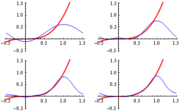
Figure 2: Successive even half-range Fourier approximations to f(x)=x^3 over the interval [0,1)